Geoff
Harries’s Web site
or
The Phoney
Photon
The reader of this site
This site is intended for readers with a good general physics background. It shows how the three effects (PE, CE and PP), can be explained in terms of waves, using “classical’ wave physics. I use concepts (radio antenna theory, information/noise theory, feedback theory), well-known to electronic engineers but perhaps not so well-known to some physicists. I include a short Tutorial.
1. Introductory notes
I use Microsoft Word. Parts of this site should appear in green or red.
Green is used to indicate a reference or some generally accepted data.
Red is an original and possibly controversial conclusion.
Black is normal linking text.
As usual, links are blue and underlined.
2. General information
Name of author - Geoffrey William Harries
Size of this file – approx. 300KB.
E-mail - Geoffharries@gmx.net
Work phone - (089) 691-22-88
Date written – May 3 2007
3. Abbreviations used in this site
CE - the Compton effect
Emr - electro-magnetic radiation
PE - the photoelectric effect
PP - pair production
PMT - the photomultiplier tube
QM - quantum mechanics
4. Site contents
The wave particle duality of light
My solution to wave particle duality>
Results of displaying this site
Miscellaneous experiments and concepts
Redefinition of Plancks constant
Introduction
A strange Effect was discovered about 100 years ago. Light, formerly thought to be a wave, was apparently behaving like a particle in what became known as the Photoelectric Effect (PE). Science tried to explain it in terms of contemporary knowledge (“classical physics”) but without success.
Einstein, using a previously discovered relation between the energy of light and its frequency, (Planck’s Constant), invented a particle whose properties corresponded to those needed. He called it the “Photon” and was awarded a Nobel prize.
The wave-particle duality of light
Since then two more effects have been discovered which science can only explain by light considered as a stream of particles (“photons”). These are the Compton effect (CE) and “pair production” (PP).
In spite of the wildly different properties of waves and particles, science has been obliged to consider that light can manifest itself as a wave or a stream of particles. This is called the “wave-particle duality” of light and has caused untold damage to science and the scientific method.
The purpose of this Site is to resolve the wave-particle duality paradox of light.
Light cannot be a wave AND a stream of particles. I must either explain all the wave properties with it as a particle OR explain all the particle properties with it as a wave.
Motivation for this site
My CV shows I am an electronic engineer. I have always felt that our brains had evolved to enable us to cope with anything we might meet in the Universe. My view is that of Rutherford who said “No physics can be good unless it can be explained to a barmaid.”
But Quantum Physics, with its complex maths and strange philosophical concepts (coherence, decoherence, Copenhagen Interpretation, delayed choice, Schrödinger’s cat, guiding waves, collapsing wave functions, Bell’s Inequality, EPR, etc. ) seemed to be an exception - a subject obviously way out of my intellectual range. Confirmed by Prof. Feynman’s notorious quotation:“The theory of quantum electrodynamics describes Nature as absurd from the point of view of common sense. And it agrees fully with experiments. So I hope you can accept Nature as she is - absurd.” Ref_6
Then I bought a book “Quantum Mechanics, Illusion or Reality?” by Alistair Rae, published by Cambridge University Press in 1998, which after the usual descriptions of mysterious phenomena ends: “One thing that should be clear is that there is wide scope for us all to have opinions and there is a disappointing lack of practicable experimental tests to confirm or disprove our ideas,” Ah! Alistair Rae is a Professor of Physics at Birmingham University and if he has doubts … So I decided to do some experiments.
Summary - science today
In 1905 Einstein invented a particle – the “photon”- to partly explain the recently discovered photoelectric effect and was awarded the Nobel Prize for it. The accepting of this invention created a discontinuity in the smoothly advancing progress of science, which even today cannot be bridged without the use of yet more mystical concepts such as “wave-particle duality”. It also gave a bad example to following scientists, who instead of grinding through what Schrödinger called the “intricacies of classical physics” when a new phenomenon is encountered, are routinely tempted to invent new concepts.
Many big brains who should be occupied in removing the need for the “photon” are instead trying to exploit its supposedly magic properties. The present condition of science can be graphically illustrated in the following picture:
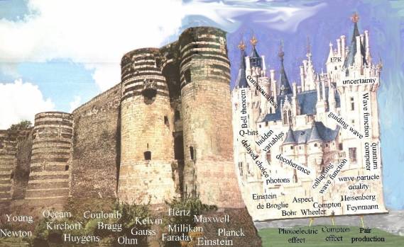
On
the left is the solid interlocking, often tested and checked Classical science,
firmly bedded in the work of the many pioneers. Shakily leaning against it is a
rococo faery castle with elaborate turrets and battlements. At its base is
marked the names of its constructors and on its ornate façade is inscribed the
names of some of the magic concepts they have invented.
Note
that this castle is supported on only three matchsticks! Three
experiments! One is called the Photoelectric Effect (PE): the other the Compton
Effect (CE) and the last Pair Production. If it were possible to explain these
three experiments in terms of Classical Physics, the whole baroque structure
would crumble. It is the purpose of this site to cut through these three
matchsticks.
My solution to the wave-particle duality paradox
I
have found a solution. It is essentially an up-to-date “classical” explanation
of that first proposed by Bohr, Kramers and Slater in their paper (around 1925).
They said, “Light of
all wavelengths behaves as a wave process (interference) with pure propagation,
but behaves as particles (light quanta, photo-effect, Compton effect) on
conversion into other types of energy”… “Light interacts with matter on a probability
basis (my italics).”
In other words, light behaves
like an expanding unquantized wave when it travels through space. But it reacts
statistically with matter, which is quantized. The greater the light’s
intensity the more probably it will react. To detect light (or emr generally)
we can only use atoms which are digital measuring instruments with quantum
resolution, and so we mistakenly think the emr is arriving in quantum sized
steps. (This is like measuring a DC voltage with a digital voltmeter having
millivolt resolution and thinking the DC voltage is quantized into millivolt
steps.)
Against this solution
Walther Bothe performed a
Nobel prize-winning experiment (based on the Compton Effect) purporting to show
this “ingenious way out of the wave-particle problem
was a blind-alley.” Ref_11
Later in this site I show that Bothes conclusion was wrong. Bohr, Kramers
and Slater were right.
Results of displaying this site
I
have shown my results to many scientists but there has been almost no response.
Most physicists are committed to wave-particle duality, they have had to
swallow it as a sort of Rite of Passage when they were undergraduates. Some
resist my solution because they have written books or papers on the subject,
others because they think they can use the magic properties of “photons” to
produce fast parallel computers or transmit data at faster than the speed of
light. Others are less concerned about the classical purity of science and say
merely “the concept works”. Still others disbelieve that so many famous
scientists from Einstein on could be proved wrong by a simple electronic
engineer.
The message behind this Site
The message of this
Site is that the behaviour of light can everywhere be explained as a wave and
so if you ever see an article or paper in which the word “photon” appears, put
that paper aside.
Logical track of this site
1. First presented is The_photoelectric_effect the interaction of emr (light) with electrons. It is conceptually easy to understand and immediately reveals Planck’s constant. I give Einstein’s explanation, using his invented particle, the “photon”, then follow it with a wave explanation.
2. Next is the_Compton_effect - also an interaction between emr (X-rays) and electrons. Very surprisingly, the wave solution of the photoelectric effect leads immediately to a simple, satisfying and obvious wave explanation of the Compton effect, leaving it otherwise untouched as a proof of Relativity. Again I first give Compton’s explanation using “photons”, and follow it with a wave explanation.
3. Third is “Pair_production” – an extension of the Compton
Effect, where very short wavelength X-rays, gamma rays, interact with matter to
produce electrons and a new particle of antimatter called the “Positron”.
4. Last covered is The_blackbody_spectrum, which is an example
of the more general interaction of emr and matter. It was the first effect to
be studied and introduced the concept of “quantum” and Planck’s Constant. It is
the most difficult to understand and so will be studied last.
For an overall picture of
how emr reacts with matter, see the Absorption_coefficient_of_lead
What I did
The keystone of the whole baroque structure seemed
to be the “photon” and so I focused all my efforts down to removing its
necessity. [After all, the purpose of science is surely to reduce the number of
axioms, not increase them.]
1.
I did many ingenious experiments (interference, refraction, non-linearity) with
laser light of all intensities using photographic films then a photomultiplier
tube as detector, and they all “supported the hypothesis” that light was a
wave. See Interference_experiments.
2. I
made a calculation showing “photons”, if they existed, were far too far apart
even in a strong laser beam to ever interact. See Calculation_of_photon_density I also show that there is normally no “photon
bunching”. So there are no “photons”.
3. If
I assumed that the free electrons in a sodium crystal behaved like the free electrons
in the carbon load of an RF dipole in the presence of emr, I could explain the
photoelectric effect using conventional RF antenna theory. And more completely
than Einstein. See The_photoelectric_effect
4. The
Compton Effect, using X-rays and first seen as a much more difficult target,
fell surprisingly easily. See the_Compton_effect.
5.
“pair production” is a strange phenomenon
showing how very high energy emr reacts with matter. Its conventional
explanation requires the emr to be quantized into “photons” and also requires
the invention of a new particle, the Positron. My classical explanation removes
at least the need for “photons”.
6. Once
the keystone of the “photon” was dislodged, the whole structure of Quantum Mechanics came tumbling down and an enormous
number of scientific papers and books
are revealed as pseudo.
The photoelectric effect
Data
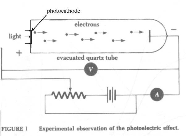
In
studying the photoelectric effect, one way is to shine light of varying
frequencies and intensities onto a thin metallic sodium “photocathode” film in
a vacuum. Nearby is a metal plate - the “anode”. The anode is connected to the
photocathode via a current measuring instrument and its voltage, with respect to
the photocathode, can be varied. In this way the number of electrons (the anode
current) can be measured. By putting different negative voltages (the “stopping
voltage”) on it, the energy of the electrons can be conveniently measured. The
higher the voltage needed to stop an electron the higher its energy. Energy
here is measured in Electron_volts or eV.
Electron volts (eV)
An electron volt is the energy gained by a particle of
charge e when it falls through a potential difference of one volt, where e is
the charge on an electron.
Energy in joules can be
converted to eV by dividing by 1.6 x 10 –19 (and vice versa). [Energy = capacity to do work.]
Background to the photoelectric effect – the sodium target
The
sodium crystal photocathode acts as an “emr energy to kinetic electron energy”
converter.
The
first reason for using a sodium crystal photocathode is that it is a way of
concentrating many electrons into a small volume. Their mutual repulsion is
nullified by the positively charged nuclei.
The
second is because the distant “free” looping electrons can be easily influenced
and detached by incident emr (light). The sodium crystal behaves like an
“opened out” sodium atom.
Thirdly,
the sodium crystal photocathode is “flat-tuned” and so can respond to emr of
any frequency within its range (unlike the sodium atom which only has definite
resonant frequencies.) See Initial_conditions_in_the_photocathode
All these characteristics facilitate the
demonstration of the photoelectric
effect.
***
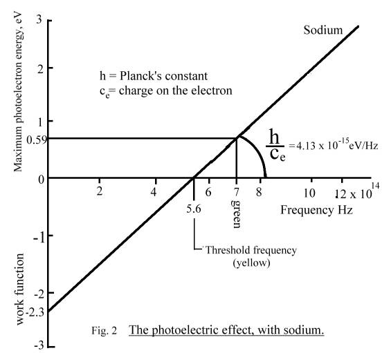
Fig. 2 shows how the energy
of the photoelectrons (in eV) varies with the frequency of the incident emr
(light) in Hz for sodium.
Note that the amplitude
of the incident light does not appear in this graph.
Work function
Even
at room temperature some electrons spring from the surface of the crystal. They
do not go far because they leave the crystal positively charged and this pulls
them back. There is therefore a negatively charged cloud of electrons
surrounding the crystal.
“There must be a minimum energy required by an electron in order
to escape from a metal surface, or else electrons would pour out even in the
absence of light. The energy characteristic of a particular surface is called
its work function.” Ref_1 Pg.45.
Fig.
2 has been extrapolated backwards to show how it intercepts the y-axis at the
work function.
Continuation of the description of the photoelectric effect
It
can be seen that if the photocathode is sodium, no electrons are emitted until
the light frequency is around 5.6 x 10¹⁴ Hz, which is yellow light.
This corresponds to a work function of
-2.3 eV which must be overcome before any electrons at all can leave the
photocathode.
Then
the energy of the emitted electron increases linearly with frequency and the
slope, the constant of proportionality, is h or 6.62 x 10⁻³⁴ joules per sec per Hz or 4.13 x 10⁻¹⁵ eV per Hz if the
energy is measured in eV.
This Constant of Nature, h,
was discovered previously by Max Planck in his study of The_blackbody_spectrum
and is called Planck’s Constant.
The
graph in Fig. 2 shows overall how emr reacts with electrons. The constant of
proportionality is h/ce, ie. :
Planck’s constant h
= 6.62 x 10 -34 =
4.13 x 10 –15 eV/Hz
Charge on an electron 1.6 x 10 -19
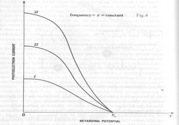
Two
other curves are required to describe the photoelectric effect. Fig. 4 shows that
photoelectric current is proportional to light intensity for all retarding voltages.
The cut-off or “extinction voltage” V0 is the same for all
intensities of light of a given frequency
“One of the features that particularly puzzled its
discoverers is that the energy distribution in the emitted electrons (called
photoelectrons) is independent of the intensity of the light. A strong light
beam yields more photoelectrons than a weak one of the same frequency, but the
average electron energy is the same. These observations cannot be understood
from the electromagnetic theory of
light. Equally odd from the point of view of the wave theory is the fact
that the photo-electronic energy depends on the frequency of the light
employed. At frequencies below a certain critical frequency, characteristic of
each particular metal, no electrons whatever are emitted. Above this threshold
frequency the photoelectrons have a range of energies from 0 to a certain maximum
value, and this maximum energy increases linearly with increasing frequency.
Thus a faint blue light produces electrons with more energy than those produced
by a bright red light, although the latter yields a greater number of them”. Ref_1 pg.42.
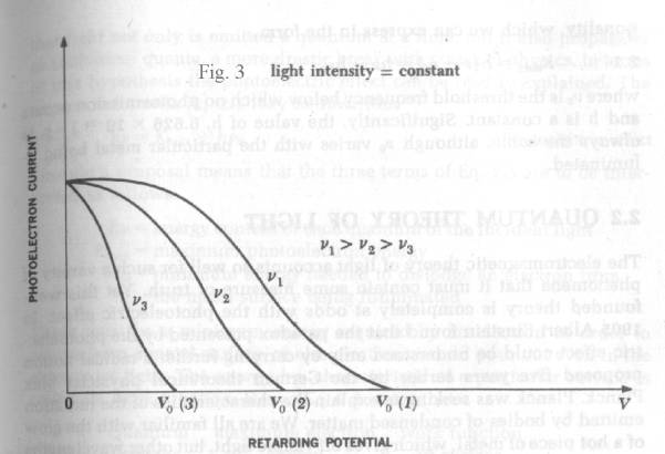
Fig .3 shows that the “extinction voltage” V0 depends
upon the frequency of the light employed.
Einstein’s explanation of the photoelectric effect
Einstein writes - “It is
clear that the relationship between Kmax (maximum photoelectron
energy) and the frequency f involves a proportionality which we can express in
an empirical formula:
Kmax = h(f - fo)
= hf - hfo
where fo is the threshold
frequency below which no photoemission occurs and h is a constant.
Significantly, the value of h, 6.626 x 10⁻³⁴ J.sec is always the
same, although fo varies with the particular metal being
illuminated.
Einstein proposed that light not
only is emitted a quantum at a time, but it also propagates as individual
quanta, (my italics) a more drastic break with classical physics. In terms of
this hypothesis the photoelectric effect can be readily explained. The
empirical formula may be rewritten:
hf = Kmax + hfo
Where hf = energy content of each quantum
of the incident light
Kmax = maximum photoelectron
energy
hfo = minimum energy needed to
dislodge an electron from the metal surface being illuminated. “Ref_1Pg. 44.
Summary of Einstein’s explanation
In
words, the incoming light must be considered as particles, as “photons” of
energy hf. A “photon” strikes a free electron in the photocathode and transfers all its energy to it. The “photon”
then “drops out of existence”.
The kinetically energized
free electron now has to fight its way out of the photocathode, losing a random
amount of energy as it bounces off the unenergized free electrons and then by
the braking effect of the Work Function barrier at the photocathode surface. It
exits the photocathode and is renamed a “photoelectron”. The energy of these
photoelectrons can be easily measured
by the voltage required to stop them and is found to be linearly
proportional to the frequency of the light producing them. Einstein received
the Nobel Prize for this interpretation.
The photoelectric effect explained with wave light
My
explanation is much more complicated than Einstein’s
but explains the effect more completely, and of course needs no
“photons.” And as Occam says ‘you should always look for a natural explanation,
however complicated, before you start inventing new phenomena.’
If
you are not familiar with the transmission and reception of low frequency
(radio frequency) emr, I suggest you click here for a short Abbreviated_tutorial
on concepts leading up to Antenna_theory.
Initial conditions in the photocathode
The standard textbook description of the metallic sodium crystal as positive ions floating in an “electron gas” is simplistic. Sodium vapour has sharp resonant peaks over the visible light range, but if it is slowly compressed in a glass tube these peaks gradually coalesce until they disappear and the metallic sodium film, now found to be formed on the inside of the tube, is aperiodic. The two far-out electrons in each sodium atom are now shared between all the atoms, linking the atoms into a sodium crystal.
These “free electrons” in the sodium film crystal must have exceedingly complicated looping orbits, winding in and out of the positive ions in three dimensions at widely varying speeds, as the radii of curvature of their orbits change and they generate and react to complex internal emr and magnetic fields. But as there are no emr or magnetic fields detectable outside the crystal, these internal “restraining fields” must cancel. Superimposed on these free electron orbits is a small thermal noise jitter. This noise jitter, being random, sometimes unbalances the restraining field and must be the reason for the occasional ejection of “thermal” electrons.
Ei = Er +
En
Where Ei =
internal field
Er = self canceling restraining field
En = thermal noise field
Widely
varying electron speeds correspond to a wide frequency range, which must be why
the sodium crystal has no tuned peaks of absorption or emission.
Note
that the thermal noise level En in the photocathode (like in a
resistor) will increase with temperature, kB, where k = absolute temperature
and B = Boltzmann’s constant.
I analyze the photoelectric effect under four Conditions:
Condition 1
See Fig. 1. No illumination. Anode at the same voltage as the photocathode. Room temperature. There is a very small current flowing between photocathode and anode. This is due to electrons which have gained enough energy through thermal noise orbit jitter, (>2.3eV = 5.6 x 10¹⁴Hz = threshold frequency for sodium = yellow light) to have escaped the photocathode through the 2.3V “work function” barrier surrounding the sodium crystal. They are called “thermal electrons.”
Condition 2
Very faint illumination by 7 x 10¹⁴Hz emr, wavelength 428nm (green, and so over the threshold frequency for sodium.)
Operation. Fig. 2 above, showing the relation between the
frequency of the incoming emr (green light) and the energy of the photoelectrons
emitted, makes no mention of the amplitude of that emr. But it cannot be zero.
Incoming wave emr must have a minimum amplitude in order to “significantly”
influence the moving electrons. In telecommunications parlance, we would say
the signal to noise ratio (SNR) must be >1. The “noise” here is the internal
field Ei, already existing in the photocathode, which is the vector
sum of the “restraining field” and random thermal noise.
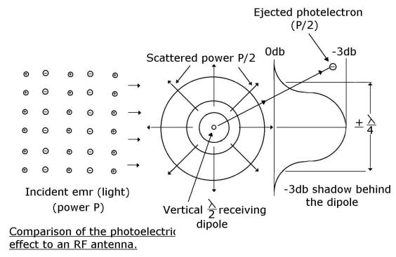
Consider a small circle on the photocathode with a radius of 107nm
(lambda/4 of green light). In the middle of this circle an electron, which by
chance has a temporary component of motion parallel to the voltage vector of
the incident green emr, behaves like a loaded dipole. Like an RF dipole, it
snaps into series resonance with the
incident emr and absorbs energy from it over the whole area of the circle,
(containing approx. 360 000 atoms if
the sodium photocathode is 1 atom thick), thereby halving its field strength,
as described under Antenna_theory, and thereby
inhibiting (or more strictly, “reducing the probability of”) any other
electrons in the circle from resonating, as the incoming emr voltage vector
amplitude applied to them is now smaller than Ei. (Remember the
incident emr amplitude has been adjusted to be just over Ei, the internal field.)
Under
the most favorable conditions, this electron exits the photocathode with a
velocity which requires 0.59V to stop it. See Fig. 2 above. Its exiting energy
is therefore 0.59eV. As it lost 2.3eV on passing the work-function barrier, it
must have abstracted 0.59 + 2.3 eV = 2.89eV from the incident emr. This amount
of kinetic energy, which we call a “quantum”, has been absorbed from the emr
and resonance is destroyed.
But
from Antenna Theory a
further quantum of energy has been reradiated or scattered from the resonating
electron, before resonance was destroyed. [This ties up with the fact
that the photocathode has been measured as reflecting 50% of the incident
light.]
In sum, a one quantum “bite” of energy of 2.89eV has been taken out of the emr wavefront leaving a
localized “hole” or “shadow” of radius 107nm. No further electrons can be
detached in the + lambda/4 circle for the moment, as the green emr field
there is now too weak (SNR < 1).
The “hole” in the field will now be
“filled” by the oncoming green emr diffusing into it. The time for it to “refill” will be inversely proportional to
the amplitude of the oncoming emr. As the hole “fills up”, the emr will again
reach the minimum amplitude necessary to overcome the internal field, Ei,
(SNR > 1) couple again with an electron somewhere in the photocathode and
produce another photoelectron. (This is analogous to a bucketful of water
suddenly scooped out of a small stream, which leaves a hole in the stream and
temporarily reduces water flow. The time taken for the hole to fill up and the
water flow to resume its former rate depends on the rate of flow, the
“amplitude”, of the stream.)
Call the following sequence
an Event -
“Incoming emr finds a resonating electron
dipole somewhere in the photocathode and transfers two quanta of energy to it.
One quantum of energy is immediately scattered from the dipole as emr. The
other quantum of energy kinetically accelerates the dipole load, the electron,
destroying the dipole and so destroying resonance. This leaves a one-quantum
energy hole in the wavefront. The accelerated electron leaves the photocathode,
its actual energy on exiting depending on its random passage through the
photocathode crystal, minus the Work Function. Pause as the oncoming emr
refills the hole. Hole filled. End of Event.”
One
Event = a one quantum “bite” taken from the wavefront. In the presence of emr,
Events are occurring continuously all over the photocathode.
Condition 3
As for Condition 2 but with greatly increased emr amplitude.
Operation. As for Condition 2, but now
slowly increase the amplitude of the incoming emr. “Events” will occur as
before, ejecting photoelectrons and producing energy holes in the wavefront,
but the greater amplitude oncoming emr will fill these holes quicker. There
will therefore be a shorter pause before the emr strength at the photocathode
rises to the minimum value (SNR=1) necessary to (probably) eject another
electron. The pause between Events is inversely proportional to emr amplitude.
There will be more Events per second,
and so anode current is also proportional to emr amplitude, as required.
Automatic gain control
It
can be seen that the average amplitude of the emr applied to the temporary
electron dipoles at any one frequency is kept constant at just over Ei,
the internal field strength, independently of the incoming emr amplitude, by a
sort of pulse-width modulated feedback loop. Standard one-quantum energy
“bites” reduce and maintain the emr amplitude at a SNR of just over 1, just
over the internal field level, Ei. The greater the incoming emr
amplitude, the greater the number of “bites” per second. The higher the
incoming emr frequency the larger the “bites.” The energy of ejected photoelectrons therefore only varies
with the incoming emr frequency and is independent of the emr amplitude,
as required.
Mathematically
Following the classical theory of free electron gas, the electrons
in a metal are free particles influenced by the incident emr:
F = -ce E
= -ce E cos ![]() t
t
where
F = force on the electron
![]() = 2
= 2![]() f where f is emr frequency
f where f is emr frequency
-ce = charge on an
electron
E = electrical field strength in volts per meter
The feedback loop
standardizes the effective incoming emr field strength in the photocathode by
width modulation to just over its internal field, Ei, adjusting it to have a signal to noise
ratio of 1.
F
= -ce E cos ![]() t where E
= 1
t where E
= 1
Ei Ei
And so the force
on the electron is only proportional to f.
The energy
given to the electron in eV, as shown in Fig. 2, is hf
ce
where f = emr frequency
h = Planck’s (empirical)
Constant, 6.626 x 10⁻³⁴
J per sec.
ce = charge on the electron
Condition 4
Incoming emr at any amplitude and at any frequency below threshold.
Operation. As in Condition 3, 1 quantum
“bites” are abstracted from the incident emr as
electrons are ejected out of their complex orbits. But the peak
kinetic energy of these electrons is too small (<2.3eV) for them to
penetrate the work function barrier so they stay in the photocathode. The
ejection of
these electrons nevertheless “loads” (takes bites out of) the emr
wavefront, limiting its amplitude in the photocathode to just above Ei,
using the feedback mechanism described for conditions 2 and 3 above. All the
ejected electrons can do now is to heat the photocathode. At very high
amplitude incident emr their energies finally start to cumulate as the “holes”
begin to overlap, producing thermal electrons at >2.3eV.
Comparison of the alternative wave explanation with the Einsteinian
The
Einsteinian explanation of the photoelectric effect requires the invention of a
“photon” which deterministically knocks out one photoelectron from the sodium
photocathode with energy proportional to its frequency. An Einsteinian Event is
where a “photon” gives up all its energy to a photoelectron and
then “drops out of existence”. The energized
photoelectron may or may not pass the work function barrier. Increased emr
amplitude means increasing the number of “photons” per second and so the number
of Events per second.
The
alternative wave explanation needs no “photon”. It uses classical radio
frequency antenna concepts throughout. By intercepting two quanta of energy
2(h/ce x 7 x 10¹⁴ )eV over an area
equivalent (with green light and a sodium photocathode one atom thick) to 360
000 atoms, I say the incoming emr
“increases the probability” a photoelectron will be ejected from
this relatively large area with an energy equal to one quantum or h/ce
x 7 x 10¹⁴ eV. The other
quantum of energy is reradiated or scattered as 7 x 10¹⁴ Hz green
emr. As with the Einsteinian particle explanation, the electron in the wave
alternative may or may not penetrate the photocathode and the work function
barrier. Increasing emr amplitude increases the number of Events by reducing
the recovery time of the photocathode.
Experimental support for the wave explanation
1 - Reflection coefficient of the photocathode
If
the free electrons in the photocathode behave like the free electrons in the
load of a radio frequency dipole, 50% of the incident energy will be scattered.
See Abbreviated_tutorial and click on Antenna_theory
So half the incident light on a
PMT cathode should be wastefully scattered. Indeed the published Quantum
Efficiency of Hammamatsu photocathodes is never greater than about 30%. Further
proof is given by the fact that the sensitivity of a reflection mode
photomultiplier tube can be almost doubled if the photocathode is covered with
an anti-reflective coating. I quote from Andor Technology (“Europhotonics” June
2005, pg. 42) where they describe one of their digital cameras …“The sensors respond to a broad range of wavelengths from
the UV to the near-IR, and the customer selects the proper antireflective
coating (my italics) to
maximize the quantum efficiency (QE) in the appropriate waveband. The BV
model’s coating produces peak QE of 95% at about 550nm and the BU2’s at about
250nm”
In other words, the 50% of
the incident emr normally scattered away is reflected back onto the
photocathode. Anti-reflective coatings support the concept of light as a wave.
For
an analogy in the world of radio frequency, think of the “director” rod mounted
a quarter wavelength in front of the receiving dipole in a Yagi antenna.
But
some PMTs are the transmission type, having a semi-transparent photocathode.
Such a one is the Hammamatsu R464, which I use. This type of photocathode
should also behave like a radio antenna, scattering 50% of the incident light.
But because of its construction, 25% should be scattered backwards (reflected)
and 25% forewords. I can only measure the part scattered or reflected backwards
and I find it to be indeed 25%, as expected. See The_reflection_coefft_of_a_PMT The other 25% presumably passes through the
semi-transparent photocathode without reacting with any free electrons. (I can
visibly confirm that light does pass through the photocathode, but I
have not been able to confirm its relative intensity as 25%.)
The
Einsteinian explanation gives no reason why
only 50% of the incoming
“photons” react with the free electrons. In the Einsteinian explanation all the
incident “photons” “drop out of existence” so the photocathode should appear
black.
2 - Temperature dependence of the photoelectric effect
“The validity of the Einstein relationship was examined by many
investigators and found to be correct but not complete. In particular, it
failed to account for the fact that the emitted electron's energy is influenced
by the temperature of the solid.” Ref_9
The alternative wave explanation relates this to the
temperature dependence of the Automatic Gain Control feedback loop. As
described above, this stabilizes the amplitude of the emr actually applied to
the temporary electron dipoles, keeping it constant at just over the internal
field, Ei, (SNR = 1). But a component of Ei is thermal
noise En, and as in a resistor the effective thermal noise (En)2
increases with the ambient absolute temperature. (En)2 =
4kTR(f2 – f1) where k = Boltzmann’s constant, T =
absolute temperature, R = resistance component of impedance and f = frequency.
3 – The Einsteinian
invention of a “designer” particle, whose properties complement the
photoelectric effect, leads to circular argument: -
The photoelectric effect is explained by assuming
light is in "photon"
particles.
The only way to detect a "photon" particle
is by the photoelectric effect.
Conclusions
An
alternative wave explanation for the photoelectric effect based on RF antenna
theory has shown that the standard Einsteinian explanation, invoking the
invention of “photons”, is an
unnecessary construct, which furthermore fails to fully explain this
phenomenon.
The Compton Effect
Now that the Photoelectric
Effect has been explained in terms of classical physics, thereby removing its
need for the concept of “photon”, I
turn to what is known as the Compton Effect (CE), after the name of the
American physicist who studied it in 1926. I will describe this very important
experiment under:
History of the CE
The tools Compton used to explain it
Compton’s Nobel Prize winning explanation of the CE.
The argument between Bohr, Kramers, Slater and Bothe
The tools I must find if I wish a classical explanation
A_classical_explanation_of_the_CE
(really a restatement of that by Bohr,
Kramers and Slater)
History
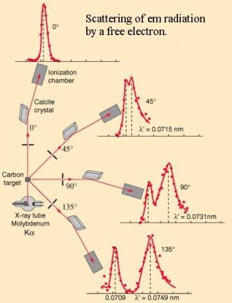
In
1926 it had been known for some time that if a beam of X-rays (the Primary Beam
or PB) were directed at a carbon target, it was scattered in a shell in all
directions with no change in wavelength, as expected. But there was also
another concentric shell of scattered radiation of a longer wavelength than the
PB, its wavelength depending on the angle with which is exited the target. See
the “Scattering of em radiation” diagram below.
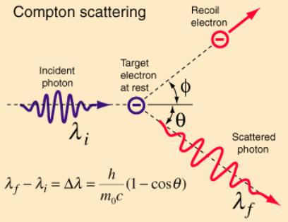
It was Compton’s
genius in finding a mathematical relationship showing that the wavelength change or shift equals h/me
c (1 – cos ![]() ), where h is Planck’s constant, me the mass of an
electron and c the velocity of light.
), where h is Planck’s constant, me the mass of an
electron and c the velocity of light.
The shift at 900
(where 1-cos ![]() = 1) is called the
Compton Shift for an electron and is 0.002426nm. Being derived from constants
it is therefore a constant itself, independent of the PB wavelength (and
amplitude.)
= 1) is called the
Compton Shift for an electron and is 0.002426nm. Being derived from constants
it is therefore a constant itself, independent of the PB wavelength (and
amplitude.)
Compton explained this
strange phenomenon using the concept of
“photon” invented by Einstein for the PE, 20 years previously. It became
known as the Compton Effect and he received the Nobel Prize for it. Because no
one over the last 85 years has found a satisfactory “wave” explanation for this
effect, it is now regarded as the strongest proof for the existence of the
“photon” and its denial is very important to my thesis.
Frequency changing (an aside)
The
Compton Effect is remarkable even from a “concept” point of view. Emr (the PB)
enters the crystal and comes out at a lower frequency, the actual frequency
depending on the angle of emission and the PB frequency.
Its
explanation is not a trivial problem and the solution is quite subtle,
requiring the PB energy to be quantized into pulses of emr before it passes
through the target. This means there are “spaces” between the pulses for them
to be “stretched into”. (Continuous emr waves cannot be stretched [reduced in
frequency or increased in wavelength]
except by Doppler shifting or using a different medium having a lower
propagation speed, neither of which is applicable here.) The reduced frequency
(“stretched”) emr pulses are produced randomly and combine statistically to
produce an output with a lower average frequency than the PB. This also
explains the observed wide bandwidth of the scattered radiation.
The
mathematical relation connecting the PB frequency, the Compton down-shifted
frequency and its angle of emission is quite complex and
by an interesting but unimportant mathematical artifact is much simpler if the
frequencies are expressed in wavelengths and the angle of emission is at 90o.
Hence the term “Compton Shift”.
[Note that the frequency f of emr is its fundamental
parameter but as it is at the moment impossible to measure it directly at such
high frequencies, wavelength, lambda, is substituted. Wavelength can be
measured with a grating and frequency is derived using f = c/lambda, where c =
velocity of light].
The Tools used by Compton
Before I reveal Compton’s explanation of the CE, I
review for you the “tools”, the concepts, he used. The most controversial is
that of the “photon”.
If the PB of frequency f is considered to be a shower of particles
called “photons”:
- this fulfils the quantization requirement allowing “stretching”. See Frequency_changing above.
- the energy associated with each “photon” is hf joules,
where h is Planck’s
Constant and f is its frequency.
- As the moving “photon” has energy, Relativity says it behaves like a
small mass and can bounce off other particles, such as the free electrons. As
with billiards, momentum and angle are conserved.
- If the momentum of a “photon” is for any reason reduced, eg. by
bouncing off and thereby sharing its momentum with another particle, its energy
and so its implied frequency is also reduced.
- “Photons” of frequency f bounce off a Bragg grating just as if they
were wave light of frequency f.
Compton’s Nobel Prize-winning explanation of the CE
The
Primary Beam, PB, “can be considered”
as a series of particles, “photons”, which strike and bounce off the carbon
target free-electrons at random angles. As an example, see below how the
electron shoots off top-right and is renamed the “recoil electron”. The
“photon”, having given up some of its energy, exits bottom right. Because it
has given up energy it now “can be considered” as having a lower frequency.
And here is Compton’s maths:
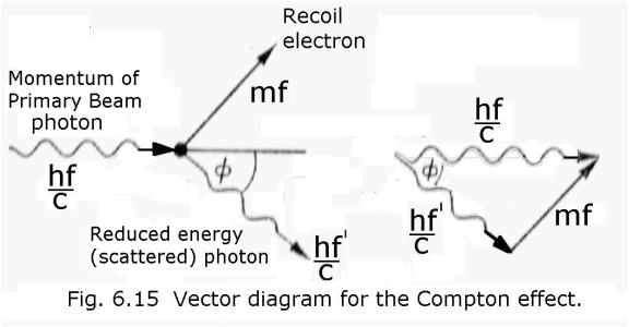
I
quote - “Quantum theory tells us that the energy of a
photon is hf and the theory of Relativity requires that we associate an energy
mc2 with a mass m. Linking these two concepts, Compton suggested
that we may put hf = mc2, which implies that the photon has momentum
mc=hf/c. The interaction between the photon and the electron may now be treated as a simple collision problem in
mechanics. The initial momentum vector hf/c (Fig. 6.15) of the X-rays is equal
to the two vectors mf and hf’/c where hf ‘/c is the momentum associated with
the scattered X-rays and mf is the
momentum of recoil of the electron. The vector triangle gives the equation:
m2f2c2
= (hf ’)2 + (hf)2 – 2h2ff’cos ![]() -------------------(6.1)
-------------------(6.1)
The conservation
of energy requires that:
hf + moc2 =
hf’+ mc2
--------------------------------------(6.2)
where mo
is the rest mass of the electron.
Relativity gives
the relation:
m2(1- f2/c2)
= mo2 -------------------------------------------(6.3)
From equations
(6.1) and (6.3) we get:
m2c4 – mo2c4
= (hf)2 + (hf’)2 – 2h2ff’cos ![]()
![]()
Substituting for
m2c4 from equation (6.2) yields
[h(f – f’) + moc2]2
– mo2c4 = (hf)2 + (hf’)2
– 2h2ff’cos ![]()
On
simplification this gives
moc2(f-f’) =
hff’(1-cos ![]() ) which becomes
) which becomes
![]() ’ –
’ – ![]() = (1 – cos
= (1 – cos ![]() ) h/moc
) h/moc
and inserting
the numerical values we get
![]() ’ –
’ – ![]() = 2.4pm when
= 2.4pm when
![]() = 90o
= 90o
which is
independent of wavelength and becomes increasingly important at shorter
wavelengths.” Ref_3 Pg.
88.
Alternatively, the frequency version of Compton’s equation
is:
1/f’ – 1/f = (1-cos ![]() ) h/mo2
) h/mo2
The CE remains
the strongest empirical proof for the
existence of a “photon” and Relativity.
Complaints from the scientific community
One of the first came
in a paper written by Bohr, Kramers and Slater in 1925. They proposed that “light of all
wavelengths behaves as a wave process (interference) with pure propagation, but
behaves as particles (light quanta, photo-effect, Compton effect) on conversion
into other types of energy”. They go on
to propose that “light interacts with matter on a
probability basis.” In other words, light normally behaves like a
wave when it goes through space but like quantized particles when it interacts
with quantized matter. [This is partly my thesis for the PE – the stronger
the light the greater the probability that photoelectrons are ejected from the
photocathode.]
Walter Bothe thought
that this could be checked experimentally and decided to do it using the CE. His “Question to Nature”
was - “Is it exactly a scatter-quantum and a recoil electron that are
simultaneously emitted in the elementary process, or is there merely a
statistical relationship between the two?” He
used two parallel detectors, one to detect the frequency down-shifted X-ray
pulses and another to detect the recoil electrons, and measured the coincidence
of the pulse outputs of these two detectors. Bothe’s
conclusion was that “systematic
coincidences do indeed occur – a scatter quantum (he meant “photon”) and a recoil electron are generated simultaneously. The
strict validity of the law of conservation of energy even in the elementary
process had been demonstrated and so the ingenious way out of the
wave-particle problem (my italics) discussed by Bohr, Kramers and Slater was shown to be a
blind-alley.” Ref_11 He received a Nobel prize for
this experiment.
This important experiment has
since been repeated by MIT using more modern equipment, and gives the same
result. Ref_12.
And so the “photon” concept
is apparently required to explain the Compton Effect.
A classical explanation of the Compton Effect
The clever part of my wave
explanation of the Compton Effect is that I very slightly modify Compton’s
method and maths but use a classical particle substituted for the imaginary
“photon”. If I want to use Compton’s maths, this classical substitute particle
must obviously have almost the same properties as the “photon” in that…
It must first be a particle.
Like a “photon”, it is produced from the incoming PB emr and its energy
depends on the frequency of this emr. (energy = hf.)
Like “photons”, the number of these particles arriving per second
depends on the intensity of the incoming emr.
Like “photons”, it must be
possible to somehow convert these particles back into wave emr of the same
frequency as that used to produce them.
Like a “photon”, its associated frequency must decrease if it loses
energy/mass for any reason, (frequency = energy/h).
Like a “photon”, it must
have momentum and so be able to bounce off a free electron in the carbon
crystal and lose energy (and thereby drop in frequency when/if it is converted
back to wave emr.)
And last but not least, it must be available in the carbon target.
I propose the photoelectron as the “classical” substitute for the
“photon” in the Compton effect.
In confirmation, let us look at the properties of a photoelectron
compared to the properties of the imaginary “photon”:
We know the energy of a photoelectron if we know the
frequency of the light producing it in the photoelectric effect. Forgetting
space charge, it is hf joules per Hz per sec. The photoelectron’s energy can be
checked in two ways:
By measuring the voltage
needed to stop it. If this is V volts, its energy is eV Electron_volts.
Alternatively the
photoelectron can be suddenly decelerated. If it is completely stopped it will
produce a burst of emr, a quantum of
frequency f, by The_Bremsstrahlung_effect.
If it is only partially
decelerated, the frequency of the burst will be < f.
And so all the qualities of a “photon” are combined in a photoelectron.
I repeat, the photoelectron is a particle and has energy (one
quantum) corresponding to the frequency used to produce it in the PE.
Relativity says it therefore has mass and
momentum which it can kinetically exchange with another particle. Any
reduction in energy corresponds to a reduction of its velocity which causes it
to emit emr (by the Bremsstrahlung effect) at a lower frequency than that used
to produce it.
Briefly, I classically
explain the CE by first dividing up (quantizing) the incoming PB by bouncing it
off the free electrons in the outer layer of the carbon target, giving
one quantum to each, using the PE.
Using Compton’s methodology, these now high-velocity, high kinetic
energy photoelectrons kinetically strike the slow-moving free-electrons deeper
in the carbon target and are deflected, sharing their energy with them, the
ratio depending on their random angle of impact. On impact they release their
reduced energy as wave emr by means of the Bremsstrahlung effect.
Essentially I take over Compton’s
calculation, replacing the fictive “photon” which carries one quantum of
energy, with a photoelectron also carrying one quantum of energy. These high
energy photoelectrons are produced inside the target.
Here is my modified vector
diagram, showing an extra stage where I
first use the PE to quantize the PB into photoelectrons: -
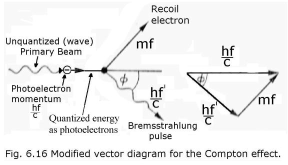
The overall principle is diagrammed below.
[Note that Bremsstrahlung is often termed the “reverse
PE.”
And as the Bremsstrahlung effect can be explained without the concept of
“photon”, the PE can too.]
My explanation of the Compton effect using Compton’s maths with photoelectrons
As there is so little
difference between mine and Compton’s explanations, I quote them together. In
order to show where I have altered Compton’s explanation, I will use my usual
colour scheme. I repeat his original words in green,
mine are in red.
“Quantum theory
(alt. The photoelectric effect) tells us that the energy of a photon (alt. photoelectron) is hf and the theory of
Relativity requires that we associate an energy mc2 with a mass m.
Linking these two concepts, I suggest that we may put hf = mc2, which implies that
the photon (alt. photoelectron) has momentum mc=hf/c. The interaction between the photon (alt. photoelectron) and the free electron may now be treated as a
simple collision problem in mechanics. The initial momentum vector hf/c (Fig.
6.15, alt. Fig. 6.16) of the X-rays is equal
to the two vectors mf and hf’/c where hf ‘/c is the momentum associated with
the scattered X-rays and mf is the
momentum of recoil of the electron. The vector triangle gives the equation:
m2f2c2
= (hf ’)2 + (hf)2 – 2h2ff’cos ![]() ----------------------(6.1)
----------------------(6.1)
The conservation
of energy requires that:
hf + moc2 =
hf’+ mc2
--------------------------------------(6.2)
where mo
is the rest mass of the free electron.
Relativity gives
the relation:
m2(1- f2/c2)
= mo2 -------------------------------------------(6.3)
From equations
(6.1) and (6.3) we get:
m2c4 – mo2c4
= (hf)2 + (hf’)2 – 2h2ff’cos ![]()
![]()
Substituting for
m2c4 from equation (6.2) yields
[h(f – f’) + moc2]2
– mo2c4 = (hf)2 + (hf’)2
– 2h2ff’cos ![]()
On
simplification this gives
moc2(f-f’) =
hff’(1-cos ![]() ) which becomes
) which becomes
![]() ’ –
’ – ![]() = (1 – cos
= (1 – cos ![]() ) h/moc
) h/moc
and
inserting the numerical values we get
![]() ’ –
’ – ![]() = 2.4pm when
= 2.4pm when
![]() = 90o
= 90o
which is
independent of wavelength and becomes increasingly important at shorter
wavelengths.” Ref_3 Pg.
88.
Alternatively, the frequency
version of Compton’s equation is:
1/f’ – 1/f = (1-cos ![]() ) h/mo2
) h/mo2
And so the result
is the same whether we use the concept of “photon” or photoelectron.
The CE is now seen as just The_Bremsstrahlung_effect,
where the electrons being decelerated
are fast photoelectrons produced inside the carbon target, rather than
separately accelerated electrons produced outside the target.
Being produced inside
the carbon target must account for the greater proportion of solid hits
with the relatively stationary free-electrons.
Comparison of the two explanations
The biggest difference is
that my explanation requires an extra stage but uses only classical concepts.
In my explanation, 50% of the
incident radiation PB is reradiated, as in the PE. This should hold for the
Compton effect too but I have not yet found anything in the literature. In any
case, reradiation is at the same frequency as the PB and it will only slightly
increase the amplitude of the normal scattered PB.
Here is my interpretation of Bothe’s experiment:
In my description of
the PE, (see The_photoelectric_effect
explanation with wave light), I say “the incoming light
increases the probability that electrons are emitted from the
photocathode”.
In exactly the same way, the
incoming PB wave in the CE is statistically quantized by the free-electrons it
first encounters in the outer layer of the carbon target. As in the PE, the
energy of the photoelectrons produced is proportional to the frequency of the
PB and their number per second is proportional to the intensity of the PB. But from here on in, the PB incoming energy has been
quantized, and the quantum pulse of Bremsstrahlung energy produced at each
impact with a free electron must obviously be coincidental with the recoil
electron. This fulfils the requirement allowing “stretching” and simultaneously
explains Bothe’s result.
So I have arrived
independently at what Bothe called the “ingenious way out of the
wave-particle problem” by Bohr, Kramers and Slater, but I can refute
Bothe’s objection to it. And therefore their way out is not a “blind-alley”. I
repeat their solution to the wave/particle duality paradox - Emr behaves
like a wave when it traverses space, but like a particle when it interacts with
quantized matter.
And so there is no
need for the “photon” particle.
Supporting my two-stage detection of high
frequency emr is Ref_14 Pg. 307 which states “An X-ray or gamma-ray photon is uncharged and creates no
direct ionization of the material through which it passes. The detection of
gamma rays is therefore critically dependent on causing the gamma-ray photon to
undergo an interaction that transfers all or part of the photon energy to an
electron in the absorbing material. …Energy loss is therefore through
ionization and excitation of atoms within the absorber material and through
Bremsstrahlung emission.”
----
Pair production (PP)
This
is the third way emr reacts with matter. The observed data is that if gamma rays of
minimum 1.022MeV enter the target, a reaction occurs in the
target and streams of two sorts of particles exit in pairs. One is an electron,
the other is a new particle, identical in every way to the electron except it
carries a positive charge. It is called the ”positron”. These particles can be
identified in a cloud-chamber and each have 0.51 MeV which is the equivalent
energy of the rest mass of an electron. Increasing the energy of the gamma rays
above 1.022MeV increases the energy of the exiting pairs by the difference. Ref_5 Pg. 140.
PP
occurs in parallel with the PE and CE. See the Absorption_coefficient_of_lead
picture below.
The
conventional explanation of PP is that the incoming Primary Beam must be
considered as a stream of “photons” and each “photon” produces a “pair” in the
high voltage field surrounding a proton. There is no explanation, classical or
otherwise, as to how positrons are actually formed.
I
need to explain pair production with classical physics and my first objection
is the use of the concept “photon”, which I hope I have shown you does not
exist. I replace the fictive “photon” by short radar-like pulses of emr
generated inside the atoms using the high speed photoelectrons already existing
in the target, produced by the PE at the target’s surface. The photoelectrons
strike the target atoms and being abruptly stopped produce the needed short
radar-like pulses of emr gamma ray pulses by Bremsstrahlung. Like science, I
offer no explanation of the conversion of these pulses into pairs.
The blackbody spectrum
It
is a strange fact that if lots of different atoms exchange emr energy with each
other, some acting as transmitters, the others as receivers, the spectrum of
their communication frequencies is the same. This “blackbody” spectrum is
obviously based on a Constant of Nature and Planck virtually by pure thought
found two things –
1. that the atoms were
communicating in short bursts of emr, now called quanta, all of different
frequencies depending on the individual atoms and how their levels of
excitation were changing.(“…coherent wave trains of 3 or 4ft. in length, as can
be observed in an interferometer”) See
2. that the energy in each
quantum was hf where f is the frequency of the burst and h is a constant of Nature,
now called Planck’s constant.
As h = 6.625 x 10⁻³⁴
joules s-1 the size of the quantized “bits” or “quanta”, are
exceedingly small, as is to be expected with atomic energy levels.
The black body spectrum is the result of “digital communication” between
atoms. Digital communication is used by Nature for the same reasons we do – to
increase the signal to noise ratio and to ensure stability. Witness
how atoms take part in the most complex electron-swapping chemical reactions
and yet emerge as atoms identical to those that entered.
Being emr and usually emitted from nearby atoms, quanta
can join up and so we normally see them as apparently continuous emr. But like
the familiar radar pulses, quanta spread out (follow the inverse square law),
getting weaker and weaker until they slide into the noise level and can no
longer be detected by any receiving atom. (If light were in particles, “photons”, they would presumably go on for ever.) It is
important to realize that a quantum is a unit of energy and not a
particle (“photon”). Einstein and Compton made this mistake and sent
Science off on a wild-goose chase which has still not ended.
For my purely
speculative idea of how atoms are constructed, see Inside_the_atom
---
Redefinition of Planck’s constant
The
importance of Planck’s Constant, h = 6.625 x 10⁻³⁴ J s-1, (called the “Quantum of action” by
scientists,) is now seen as what an
engineer would call the Coupling Factor between emr energy and matter. If the
energy is coupled to an electron, for instance, as in the photoelectric effect,
the energy coupled can be measured in Electron_volts.
The energy coupled to an electron is h/ce
where ce is the charge on the electron. For this reason the slope of
the line in the photoelectric effect is:
Planck’s constant h = 6.62 x 10 -34
= 4.13 x 10 –15
eV/Hz
Charge on an electron ce 1.6 x 10 –19
The alternative
wave explanation of the PE, CE and PP implies that Planck’s constant now needs
slightly redefining:
“h = 6.625 x 10⁻³⁴ J s for a
signal to noise ratio > 1.”
This confirms Maxwell and shows that
the power in emr is independent of its frequency and depends only on its rms
amplitude. But its Effective Power, how much of it actually couples to matter,
depends on its frequency and which matter it is coupling to. Evidence of this is seen in the increased losses in
RF components, antennas and feeders at high frequencies. Also the way the
radiated power density from an antenna increases with frequency for the same
transmitter output. For a given antenna size the radiated beam becomes
narrower. Hence the use of high frequencies for radar and long distance
communications.
As defined by Maxwell, emr is an “analog” quantity - it is not quantized.
It is only quantized by the way it reacts with
matter which is quantized.
This solves the 85
year-old enigma of how emr can behave as a wave and a particle. It does indeed
“behave like a wave when it travels from A to B but like a particle when it
reacts with matter.”
Abbreviated Tutorial
This
section may serve to remind some physicists of the simple concepts leading up
to the transmission and reception of electromagnetic radiation. Excuse me
starting from fundamentals.
Electrons
are charged particles and so can be moved by putting them in an electric field.
If electrons are moving at a constant velocity they constitute a constant
electric current and generate a constant magnetic field. This is a “Fact of
Nature”
A
piece of wire can be considered as containing
a number of “free” electrons. Under the influence of a small voltage
which provides an electric field through the wire, the electrons move and
generate the circular lines of magnetic field. The magnetic field lines push
each other apart if they are going in opposite directions.
Accelerating electrons
If
electrons accelerate they
produce electromagnetic radiation (emr). This is most easily explained by
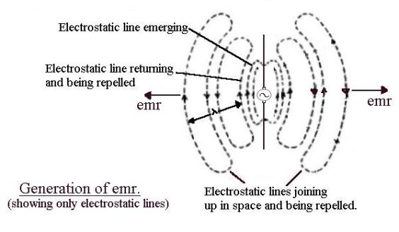
thinking of a piece of wire with a sinusoidal voltage generator in the middle. The
sinusoidal alternating voltage produces electric field lines which spread out
into space at the speed of light as the voltage increases then momentarily freeze
when maximum is reached. As the voltage drops the field lines return, finally
disappearing when the voltage is zero. The voltage now starts to increase in
the opposite direction and the field lines spread out again, this time of the
opposite polarity.
Now
think of the electrons in the wire. The electrons are pumped up then down in
synchronism with the alternating voltage. Moving electrons upwards produces a clockwise circular magnetic field
which increases as the voltage increases, expands into space, holds when the
maximum is reached, collapses to zero as the voltage drops, then expands out
anticlockwise as the electrons accelerate downwards. (Not shown in the above
diagram.)
OK
at low frequency. But now increase the frequency. As before, the field lines
expand out into space but when the polarity between the ends of the wire
change, all the magnetic and electric fields (which are limited to the speed of
light) cannot “get back” before the alternating voltage has changed over and new magnetic and electric field lines are
produced in the opposite directions. These newly generated emerging fields
“push away” or repel the inward falling field lines that have not returned “in
time”. These fields, finding themselves alone in space and being pushed away,
“join up” to form emr. These loops of electric and magnetic field, isolated in
space and propagating away from the source, are called electromagnetic
radiation (emr).
The
critical factor in their formation is the rate of change of the electric
and magnetic fields. A minimum is necessary in order to “launch” significant
emr energy. Either a low current and high frequency or low frequency and high
current can achieve this measurable minimum. In practical transmitters the
antenna current is limited so it is more profitable to operate at high
frequencies. In practice this limits
the lowest transmitter frequencies to around 10kHz.
Definition of electromagnetic radiation, emr
Emr
is a changing electric field which produces a changing magnetic field which produces
a changing electric field …Accelerating electrons are needed to “launch” emr
but once launched it is a strange self-supporting construction of electrostatic
and magnetic “field lines” which flies through space at the velocity of light.
One field “bootstraps” the other. No electrons needed!
Generating emr
Generating
emr therefore means accelerating charged particles (usually electrons) and
there are several ways of doing this.
The
way that mostly interests us is that already discussed above. A sine wave
voltage source causes the electrons in the antenna wire to move up and down.
The emr produced is at a single frequency and its amplitude, (defined in volts
per meter), depends on the amplitude of the accelerating voltage.
It
will be seen later that the power in emr depends only on its amplitude but its equivalent
power depends on its frequency as its Coupling Factor to matter ( Planck’s
constant) depends on its frequency.
Detecting emr
Emr is detected by the way it
interacts with charged particles, usually electrons because they are light and
plentiful. In order to get lots of electrons together (being negatively charged
they repel each other) we use those found in a conductor (such as a piece of
copper wire) where they are loosely attached to copper atoms and their negative
charges cancelled by the positive nucleus of the copper atoms. These
more-or-less “free electrons” are forced to follow the voltage part of the
incoming emr and moving electrons constitute an electric current, which can be
amplified. The effect can be magnified by making the piece of wire resonate at
the emr frequency. The wire is now called an “antenna”. If it is a half wavelength long, it is
called a half-wave “dipole”.
Detector noise level
Not
usually discussed in physics books on QM but very important in engineering, is
the amplitude of emr. Emr cannot be reliably detected unless it can move
an electron significantly more than that electron’s random or thermal movement. Engineers say the emr amplitude must
be above the “noise level” or signal to noise ratio (SNR >1)
Quantization of emr
As
seen above, emr can be generated in many different ways and its method of
generation determines its character. Emr generated by a continuous process, as
by the sinusoidal vibration of an electron in a radio antenna, or a laser, is a continuous or “analog”
signal. Attenuated by dispersion it can
take all amplitudes down to zero.
Such emr is not quantized – it is not in pulses or particles.
However in practice it usually appears quantized because of the way it
interacts with matter, which is quantized. For example, if an atom is
used as a detector, the electron can only take certain definite orbits or
energy states. A similar error would be
made in the laboratory if an analog voltage (which can have any value) were
measured with a digital voltmeter.
But
emr which is generated by a discontinuous process, as for instance when an atom
drops down from a high energy state to lower energy state, appears as a burst
of emr – whose frequency corresponds to the energy change (f = energy change/h,
where h is Planck’s constant.) But such emr is still an
analog pulse, like a radar pulse. And like a radar pulse it will disperse with
distance and its amplitude follow the inverse square law. Emr, however it is
generated, is a continuous wave or “analog” signal. A further important
comparison between an atom used as a quantizer for emr and an Analog Digital
Converter instrument used to measure an analog voltage, is that the amplitude
of the signal being quantized in either case must be greater than the
quantization interval. For example, a digital voltmeter which digitizes to 1mV
resolution will not notice an analog voltage whose amplitude is <1mV.
We
will see later that the size of the quantized “bits” or “quanta”, are
exceedingly small, as is to be expected when they are determined by atomic
energy levels.
In
brief, non-quantized emr is quantized by quantized matter.
Absorption of emr
If
electrons are in some way hindered in their movement (by being in soot, for
instance), energy is absorbed. The energy, which heats up the soot, is absorbed
from the emr, which is therefore weakened. In a radio antenna, where we want to
extract the maximum energy from the emr, we must connect it somehow to a load
and “match” this load to the source.
Alternatively, the emr can
be absorbed in a molecule and cause it to “rearrange” itself. Subsequent
chemical treatment reveals which atoms have received emr over threshold and
been rearranged. This it the principle of photography and farming.
Attenuation of emr
I
use this to mean some system which inputs emr at one power level and outputs it
at a lower power level. There are several ways to construct an attenuator.
Attenuators
use combinations of absorbers and dispersers. Pure dispersion could be with a
lossless convex mirror or a concave lens. Pure absorption would be a lossy
plane mirror or an absorbing medium. A convenient example is a piece of black
overexposed photographic film.
Absorption is easy to
explain if emr is considered as a wave. Electrons in the absorbing material
behave as loaded dipole antennas. They vibrate in sympathy but because they
cannot move freely they reradiate less energy than they receive. The surplus
energy heats up the absorber.
Reflection vs. scattering of emr
If
light is shone on a clean polished surface it reflects geometrically. On
a greasy or rough surface it scatters randomly. Fundamentally this is
because both surfaces contain electrons which vibrate up and down sinusoidally,
following the voltage vector of the incident emr and reradiate it. The polished
surface has many nearby (within lambda/2) electrons which also vibrate and
reradiate. Their reradiated outputs are in phase and so recreate and merely
deflect the incident wavefront.
If
all these electrons were in some way
slightly inhibited in their movements (like being tied to an atom) so
they reradiated less than they received, the reflection would still be
geometrically clean but weaker.
If the other electrons were at random distances, there
would be no combination of their outputs, each would be a point source and the
incident wavefront would be scattered.
The
key difference between reflecting and scattering is the distance between the
electrons. At a low frequency a surface often reflects – at a higher frequency
it usually scatters.
Antenna theory
One of the important sections of this paper is to convince you that the PE can be explained with the classical concepts of emr as a wave.
There is a large body of
information on long-wave emr or radio waves.
I argue that anything
that is valid for radio waves must be valid for light waves and ultimately
X-rays. Studying the large structures (antennas) used to launch and receive
radio waves must surely give us an insight into the behaviour of small
structures (single moving electrons) used to launch and receive light waves.
Transmitting or launching emr
The first and simplest way is where a sine wave voltage source causes the electrons in the antenna wire to move up and down. The emr produced is at a single frequency and its amplitude, in volts per meter, depends on the amplitude of the accelerating voltage. See accelerating_electrons
Receiving emr
Receiving
emr is much more complicated. By “receiving” is meant converting the (say
100MHz) emr wave signal which is flying
through space into a 100MHz sine-wave current in the antenna load resistor and
examining it to see if it is carrying
any signal. Like being switched off and on in the Morse code.
Now there are many types of
receiving antennas and they all have different characteristics. The only one I
am interested in here is the simplest one, the “half-wave dipole”, as I think
this one can be compared to how free electrons behave in the photocathode of
the photoelectric effect. I will therefore describe it in detail.
The half-wave dipole
The
half-wave dipole is a piece of wire, one half-wavelength (lambda/2) long, cut
in the middle and the two halves joined by a load resistor, RL. RL = 72 ohms. Placed in an emr
field of frequency f and amplitude E volts per lambda and lined up with the
electric field lines, it behaves like a signal generator of voltage E with an
output impedance of RR, the antenna’s “radiation resistance”. In
order to extract the maximum power from the receiving antenna it must therefore
be loaded (matched) with a resistance equal to
RR.
From classical antenna
theory:
1.“Total power in
watts abstracted from a radio wave by an antenna:
= (Eh)2
RL + RR + Rl
Where:
E
= field strength (rms value) of the radio wave in volts per meter
h = effective
height of the antenna in meters
RR =
radiation resistance
Rl =
antenna loss resistance
RL=
antenna load resistance
The fraction RL /(RL
+ Rr + Rl ) of this total energy represents the portion
of the abstracted energy which is usefully employed. Of the remainder, part is accounted for by the
antenna losses, such as wire and ground resistance, while the
rest is reradiated or reflected. Ref_10 Pg. 654
2.“The maximum
amount of energy that it is theoretically possible for a given antenna to
abstract from a passing radio wave occurs when the antenna loss resistance is
negligibly small and its load resistance RL is equal to the
radiation resistance. Under these conditions the rate at which energy is
abstracted from the wave is:
E2 watts where E
= rms field strength in volts/meter.
2RR RR = radiation
resistance
3. “The
reradiation of energy results from the fact that, when current flows in an
antenna, radiation takes place irrespective of whether the voltage producing
the current is derived from a passing radio wave or from a transmitter tube.”
Ref_10 Pg. 654
So only E2 watts is available as
useful power to the antenna load
2 RL
4.
Furthermore, “Calculations
show that a section of wavefront extending for only about one-quarter of a wavelength on each
side of the receiving antenna will be capable of supplying the received energy.
Analysis shows that the effect of the receiver antenna on the
passing wave is, first, abstraction of energy which weakens the main wave, and
second, reflection or reradiation of energy, which redistributes the energy of
the passing wave in a manner depending upon the antenna tuning.” Ref_10 Pg. 655
Summary
In words, the half-wave dipole behaves like a tuned concentrating lens, focussing
and matching half the incident energy over an aperture of + ¼ lambda
onto the load resistance RL. The other half is reradiated/scattered.
There is therefore a + ¼ lambda, –3db “shadow” directly behind a loaded
half-wave dipole. Pictorially the position is as shown below:
And so the field strength
far behind a row of receiving antennas is uniform but weaker than that in front
of them. Uniform because the small discrete shadows behind each antenna have
disappeared (been smoothed out) as the oncoming emr has diffused around them.
The Bremsstrahlung effect
Electrons
can be given a high velocity by putting them in an electrostatic field. If the
electrons are now decelerated suddenly by firing them at a piece of metal,
they produce a cone of wide bandwidth
emr called “Bremsstrahlung.” This is how X-rays are produced. The highest
frequency produced, due to a solid hit with a metal ion, is eV/h. Lower
frequencies are due to glancing hits.
The
Bremsstrahlung effect is the exact opposite of the PE. Instead of emr
accelerating (photo)electrons, decelerating electrons produces emr. To quote “when an
electron loses a large amount of energy by being decelerated, an energetic
pulse of emr is produced.” Ref_5 Pg. 138
For this reason the Bremsstrahlung
effect is often termed the “reverse PE.” And as the Bremsstrahlung effect can
be explained without the concept of “photon”,
the PE can too.
***
Absorption coefficient of lead
The
three ways in which emr reacts with matter overlap at different frequencies, at
different energies, as shown below: Ref_5 Pg. 177.

Interference experiments
Having shown that the
photoelectric effect can be
explained with classical physics, see The_photoelectric_effect,
I now describe a series of experiments which constitute the second half of my
argument. The results of these experiments can best be interpreted by
considering light to be a wave. And I postulate that if
light behaves like a wave it cannot be a particle - the properties are too
different.
Concept of “Gradualism
The following test was
designed using the concept of “gradualism”.
Many experiments are described in popular books on QM where first strong
light is used and visibly behaves like waves. Then this light is attenuated and
the experiment repeated using a sensitive light detector such as photographic
film. Now the results are described in terms of light as particles. Strong
light is supposed to display the characteristics of waves whereas weak light the characteristics of particles.
The idea behind my version of these experiments was that it should be possible
to slide slowly from strong light to weak light and see one characteristic
slowly blend into another. A key factor is the way the strong light is
converted into weak light – the attenuation method.
Bunching
At the time I was testing an
ingenious theory that wave light was constructed of individual hooked-together
“photons”, in the same way a piece of metal is constructed from hooked-together
individual atoms. Attenuation was imagined as pulling the “photons” apart but
leaving random “bunches” of still connected “photons”. These bunches of
“photons” would exhibit the wave
properties seen for example in Youngs_two_slit_experiment
with weak light. The problem was to design experiments which should
differentiate between wave and particle light and then perform them with strong
and weak light, using different types of attenuators, and see if there was any
difference.
The first experiment will make
the idea clear.
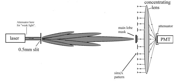
Experiment 1
Shine
an unattenuated laser onto a 0.5mm single slit and observe the sinx/x pattern on a distant screen. Now put a lens
in front of the screen to collect the entire pattern into a single bright dot.
Shine the dot into a PMT
desensitized with an attenuator in front of it to protect it and also so it has
a reasonable (say) 100kHz count rate.
Now place a mask in front of
the lens so only light from the side lobes of the sinx/x pattern enters the
PMT. The main lobe is screened out. The count rate drops to C1. Note C1.
Place
a different mask in front of the lens, this time screening out all the side lobes.
Only the main lobe passes. Note the count rate, C2.
Compute C1/C2 which
represents the ratio of light in the side lobes to the light in the main lobe
for strong light.
Remove
the attenuator in front of the PMT so it now has its normal full gain.
Repeat
the experiment with some sort of attenuator directly in front of the laser to
produce “weak light” (average 1000 clicks per sec.) and compute C1/C2 again.
The
rationale behind this experiment was the idea that more “weak light”, which was supposedly
“photons”, would go straight through the slit into the main lobe, (like
golf-balls, as the popular-science books say)
and not be diffracted into the side lobes. This would be confirmed if
the C1/C2 ratio decreased as the light was made weaker.
I used different
types of attenuators as I was looking for evidence to support my wave/particle
duality “clump” theory (now abandoned). These attenuators were usually 10mm disks punched out of
overexposed photographic film but also crossed-polarizers and band-pass filters
operated far outside their band.
Result
There was no change in the
C1/C2 ratio.
Conclusion 1– This
result is consistent with the concept of weak light
as a wave. Therefore there are no “photons”.
Conclusion 2 – This result also helps the understanding of an
“emr attenuator”. It shows that the attenuators I used behaved as they should
if emr could be considered as a wave. They reduced the size of the E and B
vectors, presumably heating up in the process, in the same way they work in wave
guides. The greatly attenuated light was still coherent. But if emr is
“photons” they would act as “dividers” ie. 1000 photons per second “in” and 1
“photon” per second “out” means an attenuation factor of 1000. And if emr is considered as “photons” each
attenuation method requires a different exotic explanation. All the attenuators
I used could be simply explained by considering emr to be a wave and Occam says
we should take the simplest explanation and “not multiply our entities”.
Other experiments I have done
The
logic behind most of the following experiments is that “weak light”, which
gives a small number of “clicks” per second when measured with my PMT, may be
“photons”. But if this weak “photonic” light behaves exactly like regular
“strong” wave light, the concept of particle light is wrong. I.e. there is no
need for “photons”, there is just weak
wave light.
Experiment 2 (This is similar to Experiment 1)
I wanted to measure numerically the beam profile of my
laser and so fitted my PMT with a 0.5mm wide vertical slit mask. I covered the
slit with an “over-exposed film” attenuator, otherwise the laser would have
damaged the PMT.
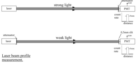
A. I mechanically scanned
the PMT across the laser beam in 0.5 mm steps, noting the PMT count rate at each
step. Distance between laser and PMT
2m. The count rate in the beam was 1kHz. I then drew the beam profile,
which was about 5mm wide. This diagram confirmed what my eyes saw.
B. Now I wanted to repeat
this experiment using attenuated (“weak”) light (possibly “photons”.) To do
this I would have to attenuate the laser and return the PMT to its normal
sensitivity by removing the attenuator from in front of it. What more natural
than to remove the attenuator from in front of the PMT and place it in front of
the laser? Working in complete darkness I now repeated step A.
Results
The count rate per step was approximately the same
and the beam profile unaltered at a sharp 5mm.
(Intuitively there should be
no difference. All we have done is changed the position of the attenuator in
the beam – from directly in front of the PMT to directly in front of the laser.
Out of curiosity I placed the attenuator in the beam half-way between the laser
and the PMT and as you might expect, it made no difference.)
Comments
Again
the problem with attenuators if light is considered as particles.
The input to the attenuator
is the output of the laser and is surely wave light as it produces interference
patterns. How does the attenuator work? Two possible methods:
1. The film attenuator
“somehow” converts or quantizes its high-power wave input into 1 000 “photons”
per second which individually knock 1
000 photoelectrons per sec from the PMT photocathode.
2.
The film attenuator weakens its input by resistive absorption,
reducing the size of the E and B vectors and so heating up. The output is low
amplitude wave light whose amplitude “increases the probability of electron
ejection” in the PMT photocathode to the point that 1 000 electrons per sec.
are ejected.
Conclusion
Explanation 1 requires an attenuator capable of “somehow” converting or quantizing wavelight into particle light. Explanation 2 uses a standard component. The wave light explanation is more convincing. And so there are no “photons”
Experiment 3
I
shone attenuated white light (10 000 clicks per second) through a 80nm wide
green pass-filter into my PMT and noted the average count rate. (Incidentally,
this filter works by interference, by internal reflection between several
carefully spaced half-silvered surfaces.) I then replaced the green filter with
one of exactly the same pass frequency except that it is 8nm wide. The average
count rate was 10 times smaller. These counts correspond to the areas under the
filter response curves, as would be expected if the light were a wave. I cannot
reconcile this result with the particle picture of light. The energy in a
“photon” is supposed to be that of a “quantum”, hf joules, where f is the
frequency. Surely there is an infinite number of “photons” in wide-band light as
there is an infinite number of
frequencies?
Conclusion
The simplest explanation is that weak light is a wave and so there are no “photons”.
Experiment 4
The
beam-width of a radio frequency dish antenna is given by the well-known
rule-of-thumb formula:
b = 70 lambda
d
Where b = degrees between half- power points
d = reflector diameter in wavelengths
lambda = wavelength of the emr
And so for lambda = 600 x 10-9
m and d = 0.4mm, (my red pointer laser shone through a 0.4mm slit) the
beamwidth should be 0.120.
The width of the main lobe
was actually measured at 0.0950
Conclusion
With only a small error the laser beam is behaving as it should for wave light. So there is no need for the concept of a “photon” to explain this result.
Experiment 5
a. Shine strong light from a laser onto a screen. Note the impact point. Now put a prism in the beam to refract the beam through some angle theta. Note the new impact point. Scan the screen with a movable PMT (with attenuated input to prevent damage). The count rates confirm what the eyes see – all the laser output has been refracted through an angle theta.
b. Darken the workplace, remove the attenuator from in front of the PMT and attenuate the laser beam until it makes 100 clicks per second when shone into the unattenuated PMT. Now scan the screen again with the now unattenuated input PMT.
Result
– all the light was refracted through angle theta even though the PMT is registering only 100 clicks per sec. [Refraction of light can be compared to a line of soldiers marching in step, arms linked, across a field. The soldiers on the left encounter a muddy patch and slow down, causing the whole line to pivot anti-clockwise to the left. If the soldiers were not linked, the line would just break up, all the soldiers marching straight on forwards individually at different speeds. And so unconnected “photons”, if they exist, would merely slow down but not change direction.]
Conclusion
– This result is adequately explained by the concept of light as a wave. Weak light refracts just like strong wave light and so there are no “photons’.
Experiment 6
I
have a green laser, which works by doubling the frequency of a IR laser in a non-linear crystal. I am quite
familiar with waves being deformed and producing harmonics by a non-linear
device. But what does non-linearity mean in terms of photons?
Conclusion
Light is surely behaving like a wave here. And if light is a wave there are no “photons”
Further experimental data supporting the wave theory of light
In the Bremsstrahlung effect, constant velocity
electrons are suddenly slowed down or
decelerated in a block of metal. Emr over a wide bandwidth is produced. The
highest frequency produced depends linearly on the voltage accelerating the
electrons (their velocity) and the constant of proportionality is h/ec
where h is Planck’s constant and ec is the charge on an electron.
Make a film of this and play it back in reverse. Wide bandwidth emr is focused onto a block of
metal and electrons are emitted. This is the same as the PE and for this reason the Bremsstrahlung
effect is often called the “reverse PE”.
Note that the concept of “photon” is not required to explain Bremsstrahlung. And
therefore not for its reverse, the PE .
Youngs two slit experiment
Almost every book on quantum
mechanics contains this picture:
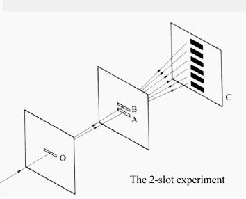
“Strong light” is shone
through slit O and then spreads out to cover slits A and B. The light from A
and B spreads out even more and overlaps. The waves beat, producing a wave
pattern on the screen C. The following diagrams show more exactly what is
happening:
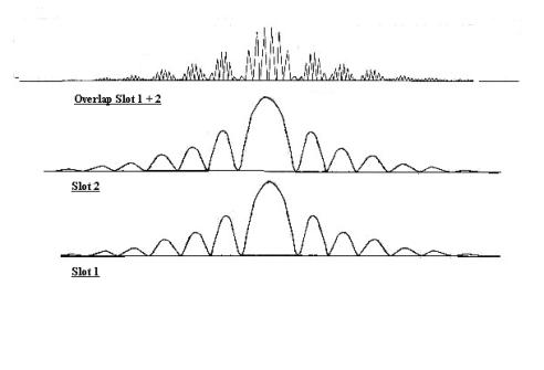
If
you believe that light is a shower of
particles (“photons”), it is possible to attenuate the light so much
that it consists of (say) 1 particle or “photon” per second. You think you have
done this because your light detector gives 1 click per second if it is a PMT.
Or before the invention of the PMT, say 50 dots on a sensitive photographic
film in 50 seconds.
Now
darken the workplace and replace the screen C with your light detector – for
example a piece of photographic film. After say 50 seconds exposure remove the
film and develop it. It looks like “50” below. Repeat the experiment with
another piece of film but make the exposure times 200 and 2000 seconds. The
developed films look like “200” and “2000” below.

This
experiment was designed to illustrate how very weak light, which is supposedly
just particles, produces a dot interference pattern on the film – one particle,
one dot. So there are 50 dots in 50 seconds, 200 in 200 seconds and 2000 in
2000 seconds. BUT – even though the “photons” are supposedly single entities
flying through space one at a time, kilometers apart, it is amazing to see them
form an interference pattern – as though they were waves! Even more amazing is
how physicists have misunderstood this
experiment. The core of the misunderstanding is that the available light
detectors (the molecules in the film, in this case) are digital detectors – they quantize the analog light falling on
them.
And so when I do Young’s
experiment with weak light (say 100 clicks per second as measured with a PMT)
it is not being done with 100
“photons” per second, but with weak
wave-light which has “increased the probability” that the photocathode will
produce an average of 100 photoelectrons per second.
Covering one slit
to try to find which “photon” went through which slit will of course destroy
the complex double-slit interference pattern and leave the simpler single-slit
sinx/x interference pattern due to the other slit. (This is sometimes
incorrectly reported in popular books as a vertical bar behind the uncovered
slit.) Nature is not trying to stop mankind from finding through which slit the
“photons” are passing - there are no “photons”, only weak wave-light which
divides itself evenly between each slit. The same applies to any experiment
where you think you are working with “photons”. [Incidentally, Young’s two-slit
experiment is overly complicated if you are testing to see if light is a wave.
A single slit is adequate – the incident light reflects off the edges of the
slit and spreads out, overlapping on the screen.]
A
point I am making here is that building comparators to correlate “clicks”
between the outputs of PMTs behind each slit in “weak light” experiments is
meaningless. You are just finding accidental correlations between random
pulses. An amazing number of experiments are done with PMTs assuming a “click”
is a “photon”, and they are all wrong.
Of course there is nothing wrong in correlating “clicks”
if the signal to noise level is over 1
(SNR>1), as in the Cerenkov flashes from underground neutrino detector
pools.
*****
CV
|
Geoffrey William Harries, Welsh father, English mother.
Born in Liverpool, England. As a little boy fascinated with radio, bought and
renovated old “crystal sets”, then built 1,2,3 valve “wireless sets”. Went to a
Grammar school until 18 or so and was usually at the top in science subjects.
Six years Military Service in the Royal Air Force in “Ground Radar”, becoming
an instructor. Through correspondence courses he obtained a City and Guilds of
London Technological Certificate. Leaving the RAF he was offered a job in the R&D
department of Marconi’s in Baddow, Chelmsford. After 5 years, married a local
girl and emigrated to Canada and worked in the R&D department of Canadian
Marconi in Montreal. Emigrated to the US after 3 years and worked in a small
company (Applied Science Corp.) in Princeton NJ which made telemetry equipment
for the US space program. Awarded two patents. Then helped form a start-up,
Applied Electronics Inc. ( See below an extract from this company’s brochure.)
After three years, divorced and with the custody of his now 6-year old eldest
daughter he returned with her to Europe and worked for 2 years at Schlumberger
in Paris in International Sales. Then he went back to Engineering in a small
French company and when this company folded became an independent importer and
consultant, finally moving to Munich, Germany, where he now lives, retired. His
life has mostly been driven by a desire to do unusual things, to solve problems
“his way”. And on the health front “no pain, no gain”. He describes himself as
a Hardware Aerospace Electronic Engineer. He would like to think he is not a
crank, but admits that after a few beers he does get philosophical. To his surprise he has
discovered in himself an almost spiritual streak, where clean
corruption-free Science is the only thing
really worth doing. This project is mostly motivated by the desire to uproot
what he considers a heresy.
|
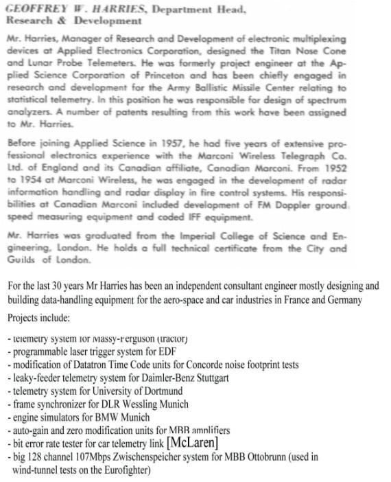
-----------
Miscellaneous experiments performed and concepts explored in the preparation of this site
Collecting information for this Site required performing unusual experiments and thinking about concepts which seem to have been too hastily accepted by Science. Coming from a different background, my views may have some interest for you.
1. Calculation of photon density in the beam of a red “pointer” laser.
3. The Heisenberg uncertainty principle
4.The wave particle duality of electrons
5. The reflection coefft of a PMT
Calculation of photon density in the beam of a red laser pointer
I look up the definition of a “photon” in the McGraw-Hill Technical Dictionary I read: -
“Pho’ton - A
single mode or polarization of the electromagnetic field. There are also two
other definitions of photon in use, not entirely consistent with the first
definition or each other: an elementary light particle or “fuzzy ball,'' and an
informal unit of light energy. The fuzzy-ball definition emphasizes the
particle character of light suggested, for example, by momentum exhibited in
the Compton effect and light levitation phenomena. However, the fuzzy-ball picture lacks a rigorous
foundation and is not required for the explanation of any fundamental
phenomenon. (My italics) As an informal unit
of energy, the photon equals hv, where h is Planck's constant (= 6.626 x 10 -34
joule-second or watts), and v is the frequency of the light in hertz.”
Hardly a very sharp-edged definition.
Now
Young’s two slit experiment demonstrates interference, and therefore the wave
nature of light, by beating together widely separated parts of a coherent
wavefront. The Calculation below shows that light considered as
"photons", even in strong light
(the output of a 1mW red “pointer” laser which is stronger than sunlight) are
on the average 160 wavelengths apart! It is difficult to see how these
“photons” could ever interfere, as they must hardly every meet – the figures
are even more outrageous as the beam is attenuated into “weak light” (and still forms an interference pattern!) Of
course it is difficult to say how a speculative particle like the “photon”
behaves, but for the dipoles in an antenna array to usefully combine their radiation,
they are in general never more than half a wavelength apart.
The calculation
A
green 500nm “photon” corresponds to: (frequency x Planck’s constant) joules.
= 0.6 x 1015 Hz x 6.62 x 10-34
= 4
x 10-19 joules
So 1mW of green light = 10-3 / 4 x 10-19
= 0.25 x 10¹⁶ “photons” per sec.
Assume the laser aperture is
4mm x 1mm and it is switched on for 1 second. The output is a thin beam 1
light-second long whose volume:
= (4 x 10-3
x 10-3 ) x (3 x 10⁸ ) m3
= 12 x 102
m3 (or 1200 cubic meters)
So the average volume
occupied by each “photon”:
= volume of 1 sec. laser
beam/number of “photons” in it
= 12 x 102 / 0.25 x 1016
= 48 x 10-14 m3
Assume for a moment the
“photons” are points and each “photon” is sitting in the middle of this
“average” volume. For ease of calculation imagine this volume is a cube of side
D. Then:
D3 = 48
x 10-14m
= 480 x 10-15 m
D
= 7.8 x 10⁻⁵ m
= 7.8 x 10-5 x 109 nm
= 78 000 nm.
So the “photons”, considered as points, are 78 000nm apart. But “photons” are described in the McGraw-Hill Technical Dictionary – see above - as “A single mode or polarization of the electromagnetic field” and so must have a dimension of lambda (in all dimensions). And as the wavelength of green light is 500nm these “photons” are:
=
78 000/500 wavelengths apart
= 156 wavelengths
Conclusion
The concept of “photon” must be wrong. So there are no “photons”.
Reflection coefft. of a PMT
The
following experiments show two independent methods of measuring how much of the
incident light is reflected from the photocathode of a transmission type PMT
(with the PMT “dead” – not connected to any counting circuitry.).
Method 1
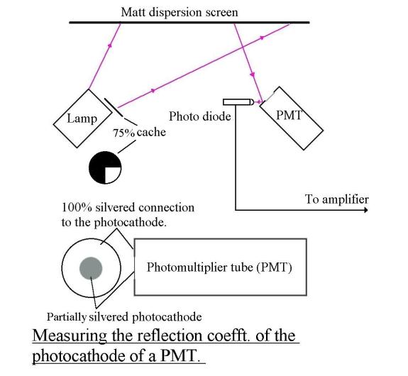
The PMT used is as
illustrated. It is a transmission type – Hammamatsu type R464. It has a glass
envelope and I use the fact that most of the end of the PMT is like a mirror,
with a 10mm diameter circular section which is the semi-transparent
photocathode. I want to measure the reflection coefficient of the photocathode
which I define as the ratio:
R = Reflected light
Incident light
The reflection coefficient
of the mirrored section = 1/1 = 1.
Principle
To
measure R, diffused light of some undefined intensity A is shone on the end of
the PMT and a photodiode is used to measure the relative intensity of the light
reflected from the two sections, photocathode and mirror-like screening.
Details
1. The photodiode is first pointed at the photocathode
to detect light reflected from the photocathode. The amplifier gain is adjusted
to give full scale.
2.The photodiode is now
pointed at the mirrored section and the amplifier
output, as expected, goes
off scale. Put an adjustable cache in front of the lamp to reduce its intensity
and adjust it until the amplifier output comes back to full scale. It is found
that the intensity must be reduced to a quarter or A/4.
We can now write R x A = A/4
x 1 and so R = ¼ or 25%.
This
result supports the antenna analogy of the PE, where 50% of the incident light
is reflected and 50% used to produce photoelectrons. Here we can only measure
the 50% of the reflected light that is reflected backwards ie, 50% of 50% or
25%. See Antenna_theory
Method 2
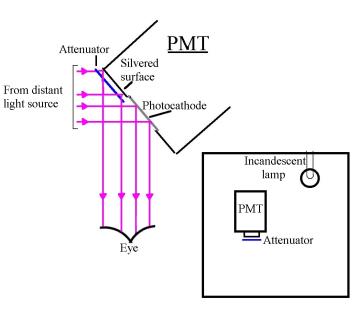
In
this method a distant light source is reflected into the eye via two parallel
paths:
reflected from a unconnected
PMT photocathode and
reflected from the silvered
surrounding of the photocathode via a
piece of attenuating film.
The attenuation of the piece
of film is selected until the two images appear the same brightness.
Under these conditions: –
A x R = A x (film
attenuation)2
(Remembering light passes through the attenuator film
twice.)
So R, the coefft of
reflection of the PMT photocathode = (film attenuation)2
R
can now be determined by measuring the attenuation of the attenuator film. This
is done in Fig. B using the PMT as a light intensity measurer and of course
connected to its normal counting circuitry.
Method
Place the measuring PMT in a light-tight box with a lamp and put a piece of the type of attenuator film as used above in front of the PMT. Adjust the lamp drive so the PMT is counting say 100 000 pulses per second. This is equivalent to the output of the lamp, bandwidth limited to the bandwidth of the attenuating film. Now put the exact piece of film used in the test between the PMT and the bandwidth filter. Without changing the lamp drive, note the PMT count. Call this C.
The attenuation of this piece of film, A is C/100 000
In practice = 50 000 so A = 0.5. The coefft of reflection
of the PMT photocathode is therefore A2 or 0.25.
In other words, 25% of the incident light on the PMT
semi-transparent photocathode is reflected: the rest passes through. This
result agrees the result obtained by Method 1.
****
Inside the atom
The hydrogen atom
The
hydrogen atom contains one negatively charged electron and one positively
charged proton. These both have the same size of electrical charge and so the
hydrogen atom is electrically neutral.
One
model (by Rutherford) of a way to keep the electron and photon apart is to have
the electron spin around the proton like a planet around the sun. If the masses
of the proton and electron and the attractive force between them are plugged
into the calculation, the dimension of the resulting structure is not far from
the measured dimension of a hydrogen atom. So this is a possible solution.
1.The first flaw in the
planetary argument is that if an electron accelerates, as it does if it is in a
circular orbit (centripetal acceleration), it radiates emr as synchrotron radiation, loses energy, slows down,
decreases orbit radius and should finally crash into the proton.
But there is no emr
radiation from hydrogen - it is a stable gas.
2.A second flaw is that if
white light (containing all frequencies) is passed through hydrogen gas, a
number of absorption lines, corresponding to many resonant frequencies are
seen. The problem is that these lines correspond to wavelengths much greater
than any possible electron orbital and so resonance frequencies of the hydrogen
atom. In particular, the lowest (red light) has a wavelength 1 500 times
greater than the hydrogen atom’s diameter!
Science has “solved” this
flaw by accepting de Broglie’s concept
of “matter waves”. The electron is considered to be a wave wrapped around the
proton.
Forced myself to invent a classical explanation of these
“flaws”, I would use the following comparison with a radio frequency
transmission line and a resonator:
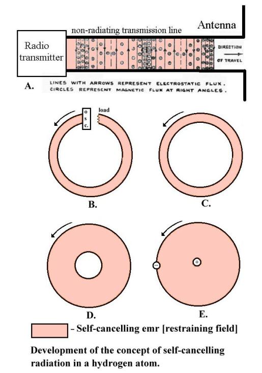
Step A. A transmitter is
connected to an antenna via a conventional transmission line. Radiation from
the two wires is self-canceling. All the emr power that is traveling along the
line is confined between the two wires.
Step B. Here a high
frequency oscillator drives a load through a looped transmission line. Again there
is no radiation as all the emr is confined between the two conductors.
Step C. Here the loop has
been cut and quickly reconnected. As the output impedance of both sides of the
momentary break match (Zo), any trapped energy will circulate
indefinitely without loss.
Step D. This is the same as
C except that the distance between the conductors has been increased by
reducing the diameter of the inner connector.
Step E. Expand this to three
dimensions with the central conductor being a reflecting point, a proton, and
we are looking at the hydrogen atom. The proton can be considered as a
ground-plane reflector. With phase reversal it reflects the emr generated by
the rotating electron. And so all the emr field generated by the orbiting
electron is confined inside its orbit. The atom behaves as a multi-mode cavity
resonator with many resonant frequencies, (Schrödinger’s equation), as familiar
in microwave technology.
Classical emr replaces de Broglie’s “matter waves”. I
invite any competent reader to tidy this up mathematically.
****
The Heisenberg Uncertainty Principle
“One of the consequences of wave-particle duality is that it sets
limits on the amount of information that can ever be obtained about a quantum
system at any one time. We can choose either to measure the wave properties of
light by allowing it to pass through a double slit without detecting through
which slit the photon passes, or to observe the photons as they pass through
the slits, so long as we sacrifice the possibility of performing an
interference experiment, but we can never do both these things at the same
time.” Or generally.. “ it is impossible to make simultaneous position and momentum
measurements on a quantum object such as a photon.” Ref. 7 Quantum_physics_illusion_or_reality
Pg. 9-10
I think the Heisenberg Uncertainty Principle is correct
but not for the reason quoted. If there are no “photons” there is no
wave-particle duality and the above statement is clearly meaningless. But the concept is familiar to anyone making
measurements.
An
example – if you want to measure a spectrum, one way is to construct a group of
contiguous filters which cover the band of interest (a “comb filter”). The
output of each filter is rectified and smoothed (integrated) to produce a DC
voltage proportional to the power in that filter. Now if the spectrum is not
completely stable (not a completely stationary series, in the jargon), you
cannot integrate for an infinitely long
time, and so the DC output of each filter will have some noise-like jitter on
it which limits the accuracy of the measurement. If you make the filters
narrower, in an effort to measure the frequencies with greater resolution, you
will find even more jitter on the filter outputs. And vice-versa, if you make
the filters wider you will find less jitter on their integrated outputs, but
you have obviously sacrificed frequency resolution. You can trade off frequency
resolution against amplitude precision.
Analytically, Shannon says the same thing. Information is
measured in “bits” and you can only collect a certain number of bits in a given
time.
Information vs. data
"The receipt of information
in the form of a message implies uncertainty in the mind of the recipient
before the message arrives. A measure of the information content of a message
can thus be based on the amount of uncertainty it has removed".
Shannon defines the Channel
Information Capacity
C = W log2
(1+S/N) bits per sec.
where W =
bandwidth and S/N = signal to noise ratio of the channel.
In
other words, you only have a limited number of bits (bits over the noise level)
available in any given time interval and so any measurement has a limited
overall precision.
If
you want to measure something that has two parameters (like frequency and
amplitude in the example above), you can “spend” these bits anyway you want –
for any ratio of frequency to amplitude resolution. But the individual precision per parameter is limited to the
number of bits you decide to spend on that parameter.
More
generally, the more parameters the measurement, the more the limited number of
available bits have to be shared out, and as the precision per parameter is
proportional to the number of bits you spend on it, the more limited the
precision per parameter.
Wave-particle duality of electrons
This
is an often quoted experiment. A beam of electrons is shone on a piece of very
thin conducting wire at right angles to the beam (the experimenter made the
wires by coating fibers from spiders' webs with gold). The electrons that pass
are allowed to strike a screen which can detect and then record the arrival of
the electrons (a fluorescent screen backed up with photographic film, for
instance). A sin x/x interference pattern builds up on the film! Even though
the electrons are only shot once per second! [This is exactly the same pattern
you see if laser light is shone through a narrow slit onto a distant screen.
Here light has reflected from the edges of the slit and is interfering with itself on the screen.] This electron
experiment is generally taken as proof that electrons, which we know (from
Millikon’s oil drop experiment) are particles, can also behave as waves.
The fine wire is supposed to be behaving like an electron biprism, splitting
each incident electron into two wave components, which then interfere with each
other.
The
importance of this notorious experiment is that it is supposed to demonstrate
the general principle that matter (in
this case electrons), can exhibit particle or wave properties. If we
accept this particular proof, where undoubted particles produce a visible
interference pattern, it can be used to support the argument that light, which
has an undisputed existence as a wave (in the 2-slit experiment), can also show
the properties of a particle. By a rather circuitous reverse-logic route we
then have a proof that light can show the properties of a wave or a
particle - ie. a proof of the existence of “photons”.
How can electrons classically behave like waves?
A
little thought shows that the electrons have random positions in the
approaching beam. Some will hit the wire head-on and won’t reach the screen.
Some will bypass the wire completely and hit the screen unaffected. But others will graze the wire at random
distances. A single moving electron, (which we know behaves like an electric
current and has a magnetic field around it),
passing the more-or-less stationary free electrons in the wire, is not
going to be unaffected. It will induce a current in the wire which will produce
an opposing magnetic field, transformer-like, and deflect the electron. And the
faster the electron or the closer the grazing, the more the deflection. And
this phenomenon can occur on a single electron-by-electron basis.
Note
that the experimenter did not use uncoated fibers. We can safely assume the
experiment would not work without a supply of free electrons in the biprism
“lens”.
To
complete my denial of this phenomena as
a demonstration of wave/particle duality, I should now make a calculation to
show the expected screen pattern. (And maybe I will in a later version of this
site.) But here I am concentrating on the wave/particle paradox of light. So I
am satisfied if I can find a rough non-mystical explanation for a phenomenon
which doesn’t directly concern me. (I invite any competent reader to tidy this
up mathematically and I will give him full credit.)
A
somewhat similar experiment was performed by Davisson and Germer in 1927. An electron beam strikes a crystalline nickel target and
bounces back at 50o if the
accelerating voltage is 54V. Ref_1 Pg. 86. The reason is surely that the magnetic fields surrounding the moving
electrons react with the regularly spaced “free” electrons in the metallic
crystal in a regular fashion. No need to invoke “electron waves”.
I
would like to expand this argument to explain the apparent self -interference
phenomena of other particles. They also surely cannot graze the atoms in their
target without being affected by them in some way. Remember we know very little
about how an atom “works”. See Inside_the_atom.
References
1.
“Concepts of Modern Physics”. Beiser. Mc.Graw-Hill. ISBN 0-07 004382-5
2.
“College Physics”. Sears, Zemansky, Young. Addison-Wesley. ISBN 0-201-07680-2
3.
“Atomic and nuclear physics”. Littlefield and Thorley. Van Nostrand.
4.
“Fundamentals of University physics”. Alonso-Finn. Addison-Wesley.
5.
“Physics of the atom”. Wehr and Richards. Addison-Wesley.
6. “QED
the strange theory of light and matter”. Feynman.
ISBN 0-14- 012505-1
7. “Quantum physics: illusion or reality?”
Rae ISBN 0-521-46716-0
8. “What
is Life?” Schrödinger. Library of
Congress 56-9403
9 .
“Encyclopedia Britannica” - Fowler
10.“Radio
Engineering”. Terman. McGraw-Hill 1937.
11. ”Nobel
Lecture in Physics 1954” by Walther Bothe.
12.
“Compton Scattering” MIT dept. of Physics. Feb.13 2004.
13. “Are there quantum jumps?” Essay by Erwin Schrödinger. Pg. 137.
Doubleday Anchor Book. US catalog card 56-9403. 1956.
14. “
Radiation Detection and
Measurement” by Knoll & Wiley
ISBN 0-471-07338-5